Non-equilibrium transitions in multiscale systems with a bifurcating slow manifold

T. Grafke, and E. Vanden-Eijnden, J. Stat. Mech 2017/9 (2017) 093208

Abstract

Noise-induced transitions between metastable fixed points in systems evolving on multiple time scales are analyzed in situations where the time scale separation gives rise to a slow manifold with bifurcation. This analysis is performed within the realm of large deviation theory. It is shown that these non-equilibrium transitions make use of a reaction channel created by the bifurcation structure of the slow manifold, leading to vastly increased transition rates. Several examples are used to illustrate these findings, including an insect outbreak model, a system modeling phase separation in the presence of evaporation, and a system modeling transitions in active matter self-assembly. The last example involves a spatially extended system modeled by a stochastic partial differential equation.


doi:10.1088/1742-5468/aa85cb

arXiv

Long Term Effects of Small Random Perturbations on Dynamical Systems: Theoretical and Computational Tools

T. Grafke, T. Schäfer, and E. Vanden-Eijnden, Fields Institute Communications, In: Recent Progress and Modern Challenges in Applied Mathematics, Modeling and Computational Science (Springer, New York, NY) (2017)

Abstract

Small random perturbations may have a dramatic impact on the long time evolution of dynamical systems, and large deviation theory is often the right theoretical framework to understand these effects. At the core of the theory lies the minimization of an action functional, which in many cases of interest has to be computed by numerical means. Here we review the theoretical and computational aspects behind these calculations, and propose an algorithm that simplifies the geometric minimum action method introduced in [M. Heymann and E. Vanden-Eijnden, CPAM Vol. LXI, 1052–1117 (2008)] to minimize the action in the space of arc-length parametrized curves. We then illustrate this algorithm's capabilities by applying it to various examples from material sciences, fluid dynamics, atmosphere/ocean sciences, and reaction kinetics. In terms of models, these examples involve stochastic (ordinary or partial) differential equations with multiplicative or degenerate noise, Markov jump processes, and systems with fast and slow degrees of freedom, which all violate detailed balance, so that simpler computational methods are not applicable.


doi:10.1007/978-1-4939-6969-2_2

arXiv

Metastability in Active Matter: Transitions between Colony Patterns in Reproducing Motile Microorganisms

Summary: Active materials can self-organize in many more ways than their equilibrium counterparts. For example, self-propelled particles whose velocity decreases with their density can display motility-induced phase separation (MIPS), a phenomenon building on a positive feedback loop in which patterns emerge in locations where the particles slow down. Here, we investigate the effects of intrinsic fluctuations in the system's dynamics on MIPS. We show that these fluctuations can lead to transitions between metastable patterns. The pathway and rate of these transitions is analyzed within the realm of large deviation theory, and they are shown to proceed in a very different way than one would predict from arguments based on detailed-balance and microscopic reversibility.

Introduction

Bacteria show complex collective behaviour. For example, bacteria such as E. Coli

  • are capable of active propulsion, i.e. have a free-swimming (planktonic) stage.
  • hey are capable of sensing their environment through quorum sensing, density-dependent gene regulation.
  • They stick to surface to form biofilms, high density colonies.
  • They exhibit cyclic/time-periodic behaviour: Biofilm formation, maturation, dispersion, planktonic stage.

The goal of this project is as follows:

Main Problem: Is it possible to describe similarly complex life-cycles as emergent behaviour of a large number of simple individual agents subject to a small number of collective rules?

Continuum description of motile bacteria

We model the motion of motile reproducing microorganisms with simple behavioural rules. The self-propulsion is modelled as active Brownian motion. For position \(X\in\Omega\subset\mathbb{R}^d\), direction \(\hat n \in S^{d-1}\), and location dependent swim speed \(v(X)\in\mathbb{R}\)

$$\dot X = v(X) \hat{n}\,,$$
$$d\hat n = \tau^{-1/2} P\circ dW\,,\qquad P=\textrm{Id} - \hat n \hat n^T$$

The direction vector diffuses on \(S^{d-1}\) with tumbling rate \(\tau^{-1}\). The fast tumlbing limit \(\tau\to0\) yields Brownian motion

$$ dX = \sqrt{2 D(X)} \circ dW $$

with density dependend diffusivity \(D(x) = v^2(x)\). Now consider \(N\) such particles with position \(X_i, i\in\{1,\dots,N\}\). To model quorum sensing, introduce scale \(\delta\) over which particles feel each other's influence,

$$dX_i = \sqrt{2 D(\rho_{N,\delta}(t,X_i))}\circ dW_i$$

with

$$\rho_{N,\delta}(t,x) = \int_\Omega \phi_\delta(x-y)\rho_N(t,y)\,dy,\qquad \rho_N(t,x) = \frac1N \sum_{j=1}^N \delta(x-X_j(t))$$

In the limit \(N\to\infty\), through a Deans-type argument, this yields a closed integro-differential equation for \(\rho_N\to\rho\),

$$\partial_t \rho = \nabla\cdot(D(\rho_\delta) \nabla\rho +\tfrac12 D'(\rho_\delta)\nabla \rho_\delta),\qquad \rho_\delta(t,x) = \int_\Omega \phi_\delta(x-y)\rho(t,x) \,dy$$

in the sense that

$$\forall\ \varepsilon,T>0:\quad \lim_{N\to\infty} \mathcal P\Big(\sup_{0\le t\le T}\Big| \frac1N \sum_{j=1}^N f(X_j(t))-\int_\Omega \rho(t,x) f(x)\,dx \Big| >\varepsilon \Big)=0$$

To make this model closed in \(\rho(t,x)\), consider \(D(\rho)=D_0 e^{-\rho}\), and expand in \(\delta\ll1\),

$$\rho_\delta(x) \approx \rho(x) + \tfrac12 \delta^2 \partial_x^2 \rho(x)\,.$$

Then we obtain an effective diffusion equation

$$\partial_t \rho = \nabla \cdot (D_e(\rho)\nabla\rho - \delta^2 \rho D(\rho) \nabla\Delta \rho)$$

with diffusivity

$$ D_e(\rho) = D(\rho) + \tfrac12 D'(\rho)\rho\,. $$

Despite the microscopic model being not reversible, the continuum model restores detailed balance

$$ \partial_t\rho = \nabla\cdot(\rho D(\rho) \nabla(\delta E/\delta \rho)) $$

with free energy

$$ E(\rho) = \int_\Omega (\rho\log\rho - \rho + f(\rho) + \tfrac12 \delta^2 |\nabla \rho|^2)\,dx\,,\quad f'(\rho)=\tfrac12 \log D(\rho) $$

In other words, the model is a \((\rho D(\rho))\)-Wasserstein gradient flow. This model demonstrates the effect of motility induced phase separation: While the microscopic diffusivity \(D(\rho)\) is strictly positive, this is no longer true for the effective diffusivity \(D_e(\rho)\)! For example, for \(D(\rho) = D_0 e^{-\rho}\), the effective diffusivty becomes

$$D_e(\rho) = D_0 (1-\tfrac12\rho) e^{-\rho}$$

As a consequence, homogeneous configurations \(\rho(x) = \bar\rho\) are only stable, if \(\bar\rho<2\). If instead \(\bar\rho>2\) phase separation occurs, as depicted in the animation. This is the mentioned feedback loop: Accumulation induced slowdown and slowdown-induced accumulation.

We now additionally introduce a second behavioral rule for the active agents: Reproduction and competition. This is models as a Poisson process

$$A\stackrel{\lambda_r}{\longrightarrow} A+A\qquad\lambda_r=\alpha\qquad\text{(reproduction)}$$
$$A+A\stackrel{\lambda_c}{\longrightarrow} A\qquad\lambda_c=\alpha/\rho_0\qquad\text{(competition)} $$

with carrying capacity \(\rho_0\) and timescale \(\alpha\). In the limit \(N\to\infty\), this effectively leads to logistic growth

$$\partial_t \rho = \nabla \cdot (D_e(\rho)\nabla\rho - \delta^2 \rho D(\rho) \nabla\Delta \rho) {\color{red} + \alpha \rho (1-\rho/\rho_0)} $$

Interestingly, now, phase separation will eventually occur if \(D_e(\rho_0)<0\), even if currently \(D_e(\bar\rho)>0\). In other words, the system will drive itself into instability. In particular, we identify three regimes, with spinodal density \(\rho_S\) and critical density \(\rho_c\):

  • if \(\rho_0 < \rho_S\), only the homogeneous solution will be stable, and no instability occurs (homogeneous phase)
  • if \(\rho_S < \rho_0 < \rho_c\), instead limit cycles occur, where reproduction induces motility induced phase separation, but the resulting dense bacterial clusters are unsustainable under the current carrying capacity, and thus slowly die out.
  • if \(\rho_c < \rho_0\), bacterial clusters become (meta-)stable.

This behavior is reminiscient of the biofilm-planktonic lifecycle: Bacteria occur in a diluted planctonic phase, until a critical density is reached. They then stick to walls to form a biofilm, which over time slowly dissolves back into the planktonic phase. The corresponding phase-diagram in carrying capacity \(\rho_0\) and inverse quorum sensing range (equivalently, domain-size), \(\delta^{-1}\), is shown in the figure.

Relevant publications

  1. T. Grafke, M. Cates, and E. Vanden-Eijnden, "Spatiotemporal Self-Organization of Fluctuating Bacterial Colonies", Phys. Rev. Lett. 119 (2017), 188003 (link)

Simplified Geometric Minimum Action Method for the Computation of Instantons

Summary: Small random perturbations may have a dramatic impact on the long time evolution of dynamical systems, and large deviation theory is often the right theoretical framework to understand these effects. At the core of the theory lies the minimization of an action functional, which in many cases of interest has to be computed by numerical means. Here, a numerical method is presented to effectively compute minimizers of the Freidlin-Wentzell action functional in very general settings. The matlab source code of the algorithm and some test problems is available for download here.

Introduction

Small random perturbations often have a lasting effect on the long-time evolution of dynamical systems. For example, they give rise to transitions between otherwise stable equilibria, a phenomenon referred to as metastability that is observed in a wide variety of contexts, e.g. phase separation, population dynamics, chemical reactions, climate regimes, neuroscience, or fluid dynamics. Since the time-scale over which these transition events occurs is typically exponentially large in some control parameter (for example the noise amplitude), a brute-force simulation approach to compute these events quickly becomes infeasible. Fortunately, it is possible to exploit the fact that the mechanism of these transitions is often predictable when the random perturbations have small amplitude: with high probability the transitions occur by their path of maximum likelihood (PML), and knowledge of this PML also permits to estimate their rate. This is the essence of large deviation theory (LDT), which applies in a wide variety of contexts. For example, systems whose evolution is governed by a stochastic (ordinary or partial) differential equation driven by a small noise or by a Markov jump process in which jumps occur often but lead to small changes of the system state, or slow/fast systems in which the fast variables are randomly driven and the slow ones feel these perturbations through the effect fast variables only, all fit within the framework of LDT. Note that, typically, the dynamics of these systems fail to exhibit microscopic reversibility (detailed balance) and the transitions therefore occur out-of-equilibrium. Nevertheless, LDT still applies.

LDT also indicates that the PML is computable as the minimizer of a specific objective function (action): the large deviation rate function of the problem at hand. This is a non-trivial numerical optimization problem which calls for tailor-made techniques for its solution. Here we will focus on one such technique, the geometric minimum action method, which was designed to perform the action minimization over both the transition path location and its duration. This computation gives the so-called quasipotential, whose role is key to understand the long time effect of the random perturbations on the system, including the mechanism of transitions events induced by these perturbations.

Simplified geometric minimum action method

Consider

$$dX = b(X) dt + \sqrt{\epsilon} \sigma(X) dW\,,$$

where \(b: \mathbb{R}^n \to\mathbb{R}^n\) denotes the drift term, \(W\) is a standard Wiener process in \(\mathbb{R}^n\), \(\sigma: \mathbb{R}^n \to \mathbb{R}^n \times \mathbb{R}^n\) is related to the diffusion tensor via \(a(x) = (\sigma \sigma^\dagger)(x)\), and \(\epsilon>0\) is a parameter measuring the noise amplitude. Suppose that we want to estimate the probability of an event, such as finding the solution in a set \(B\subset \mathbb{R}^n\) at time \(T\) given that it started at \(X(0)=x\) at time \(t=0\).

Minimization problem

In the limit as \(\epsilon\to0\), this probability can be estimated via a minimization problem

$$\mathcal{P}^x \left(X(T)\in B\right) \asymp \exp\left(-\epsilon^{-1} \min _{\phi\in \mathcal {C}} S_T(\phi) \right)$$

for the action functional (or rate function)

$$ S_T(\phi) = \tfrac12\int_0^T \langle\dot \phi - b(\phi), \left(a(\phi)\right)^{-1}(\dot \phi - b(\phi))\rangle\,dt\,.$$

Here \(\asymp\) denotes log-asymptotic equivalence (i.e. the ratio of the logarithms of both sides tends to 1 as \(\epsilon\to0\)), the minimum is taken over the set \(\mathcal{C} = \{ \phi\in C([0,T],\mathbb{R}^n): \phi(0)=x,\phi(T)\in B\}\), and we assumed for simplicity that \(a(\phi)\) is invertible and \(\langle\cdot,\cdot\rangle\) denotes the Euclidean inner product in \(\mathbb{R}^n\). LDT also indicates that, as \(\epsilon \to0\), when the event occurs, it does so with \(X\) being arbitrarily close to the minimizer \(\phi_* = \mathop{\text{argmin }} _{\phi\in \mathcal {C}} S_T(\phi)\). We can define a Hamiltonian associated with the action functional above via \(H(\phi,\theta) = \langle{b(\phi)},{\theta}\rangle+\tfrac12\langle{\theta},{a(\phi) \theta}\rangle\). Our algorithm will turn out to be valid for more than just Hamiltonians of this form.

As detailed in Proposition 2.1 of [Heymann, Vanden-Eijnden, CPAM 61 (8), 2008], it is possible to redefine the action functional to a geometric form,

$$\hat S(\phi) = \sup_{\theta: H(\phi,\theta=0)} \int_0^1 \langle \phi', \theta\rangle\,ds$$

and we abbreviate \(E(\varphi,\vartheta) = \int_0^1 \langle{\varphi'},{\vartheta}\rangle\,ds\). Let

$$ E_*(\varphi) = \sup_{\vartheta:H(\varphi,\vartheta)=0} E(\varphi,\vartheta) $$

and \(\vartheta_*(\varphi)\) such that \(E_*(\varphi) = E(\varphi, \vartheta_*(\varphi))\). This implies that \(\vartheta_*\) fulfills the Euler-Lagrange equation associated with the constrained optimization problem, that is,

$$ D_\vartheta E(\varphi, \vartheta_*) = \mu H_\vartheta(\varphi,\vartheta_*)\,,$$

where on the right-hand side \(\mu(s)\) is the Lagrange multiplier added to enforce the constraint \(H(\varphi,\vartheta_*)=0\). In particular, at \(\vartheta=\vartheta_*\), we have

$$ \mu = \frac{\|D_\vartheta E\|^2}{\langle\!\langle{D_\vartheta E},{H_\vartheta}\rangle\!\rangle} = \frac{\|\varphi'\|^2}{\langle\!\langle{\varphi'},{H_\vartheta}\rangle\!\rangle}\,, $$

where the inner product \(\langle\!\langle{\cdot},{\cdot}\rangle\!\rangle\) and its induced norm \(\|\cdot\|\) can be chosen appropriately, for example as \(\langle{\cdot},{\cdot}\rangle\) or \(\langle{\cdot},{H_{\vartheta\vartheta}^{-1} \,\cdot}\rangle\).

At the minimizer \(\varphi_*\), the variation of \(E_*\) with respect to \(\varphi\) vanishes. We conclude

$$\begin{aligned} 0 = D_\varphi E_*(\varphi_*) &= D_\varphi E(\varphi_*,\vartheta_*) + \left[D_\vartheta E D_\varphi \vartheta \right]_{(\varphi,\vartheta)=(\varphi_*,\vartheta_*)}\nonumber\\ &= -\vartheta_*' + \mu \left[H_\vartheta D_\varphi \vartheta\right]_{(\varphi,\vartheta)=(\varphi_*,\vartheta_*)} \nonumber\\ &= -\vartheta_*' - \mu H_\varphi(\varphi_*,\vartheta_*)\,, \label{eq:optim-psi} \end{aligned}$$

where in the last step we used \(H(\varphi, \vartheta_*)=0\) and therefore

$$H_\varphi(\varphi, \vartheta_*) = - H_\vartheta(\varphi,\vartheta_*) D_\varphi \vartheta.$$

Multiplying the gradient with any positive definite matrix as pre-conditioner yields a descent direction. It is necessary to choose \(\mu^{-1}\) as pre-conditioner to ensure convergence around critical points, where \(\varphi'=0\).

Algorithm

Summarizing, we have reduced the minimization of the geometric action into two separate tasks:

  1. For a given \(\varphi\), find \(\vartheta_*(\varphi)\) by solving the constrained optimization problem

    $$\max_{\vartheta, H(\varphi,\vartheta)=0} E(\varphi,\vartheta)\,,$$
    which is equivalent to solving
    $$ D_\vartheta E(\varphi,\vartheta_*) = \varphi' = \mu H_\vartheta(\varphi,\vartheta_*)$$
    for \((\mu,\vartheta_*)\) under the constraint \(H(\varphi,\vartheta_*)=0\). This can be done via gradient descent, a second order algorithm for faster convergence (e.g. Newton-Raphson) or, in many cases, analytically.

  2. Find \(\varphi_*\) by solving the optimization problem

    $$\min_{\varphi\in\hat{\mathcal{C}}_{x,y}} E_*(\varphi)\,,$$
    for example by pre-conditioned gradient descent, using as direction
    $$-\mu^{-1} D_\varphi E_* = \mu^{-1}\vartheta_*'(\varphi) + H_\varphi(\varphi,\vartheta_*(\varphi))\,,$$
    with \(\mu^{-1}\) as pre-conditioner. The constraint on the parametrization, e.g. \({|\varphi'|=\textrm{const}}\), must be fulfilled during this descent (see below).

Applications

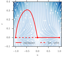
Maier-Stein model: Breaking detailed balance

Maier and Stein's model [J. Stat. Phys 83, 3–4 (1996)] is a simple system often used as benchmark in LDT calculations. It reads

$$ \begin{cases} du = (u-u^3-\beta u v^2) dt + \sqrt{\epsilon}dW_u\\ dv = -(1+u^2)v dt + \sqrt{\epsilon}dW_v\,, \end{cases}$$

where \(\beta\) is a parameter. For all values of \(\beta\), the deterministic system has the two stable fixed points, \(\varphi_-=(-1,0)\) and \(\varphi_+=(1,0)\), and a unique unstable critical point \(\varphi_s=(0,0)\). However it satisfies detailed balance only for \(\beta=1\). To the right, the transition paths between the two stable fixed points is depicted in comparison to the heteroclinic orbit. The source code for this problem is available below.

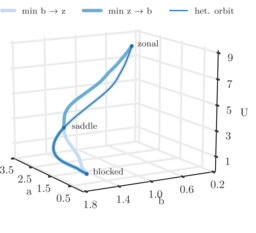
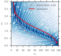
Eggers model: Meta-stable climate regimes

Egger [J. Atm. Sc. 38, 12 (1981)] introduces the following SDE system as a crude model to describe weather regimes in central Europe:

$$\small \begin{aligned} da =& kb(U-\beta/k^2)\,dt - \gamma a\,dt + \sqrt{\epsilon} dW_a\,,\\ db =& -ka(U-\beta/k^2)\,dt + UH/k\,dt \\&- \gamma b\,dt + \sqrt{\epsilon} dW_b\,,\\ dU =& -bHk/2\,dt-\gamma(U-U_0)\,dt + \sqrt{\epsilon} dW_U\,. \end{aligned}$$

When \(\epsilon\) is small, these equation exhibit metastability between a "blocked state" and a "zonal state". To the right, the transition paths between these two states is depicted in comparison to the heteroclinic orbit. The source code for this problem is available below.

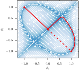
Allen-Cahn/Cahn-Hilliard model: Phase separation and growth

Consider the SDE system

$$ d\phi= (\frac1\alpha Q (\phi-\phi^3) - \phi)dt + \sqrt{\epsilon} dW$$

with \(\phi=(\phi_1, \phi_2)\) and the matrix \(Q=((1,-1),(-1,1))\). This system does not satisfy detailed balance, as its drift is made of two gradient terms with incompatible mobility operators (namely \(Q\) and \(\textrm{Id}\)). This model can be seen as a 2-dimensional reduction to a discretized version of the continuous Allen-Cahn/Cahn-Hilliard. When \(\alpha\) is small, there exists a "slow manifold", comprised of all points where \(Q(\phi-\phi^3)=0\) which is shown as a white dashed line to the right. On this manifold, the deterministic dynamics are of order \(O(1)\), which is small in comparison to the dynamics of the \(Q\)-term, which are of order \(O(1/\alpha)\). This suggests that for small enough \(\alpha\) the transition trajectory will follow this slow manifold on which the drift is small, rather than the heteroclinic orbit, to escape the basin of the stable fixed points. This intuition is confirmed in the plot to the right. The source code for this problem is available below.

Genetic switch: A non-quadratic Hamiltonian

The algorithm can readily be applied to situations, where the Hamiltonian is non-quadratic. This is the case for example for birth-death-processes with a positive feedback loop, modeled as continuous time Markov process. The model

$$ \begin{aligned}H(\phi,\theta) &= \frac{a_1}{1+\phi_b^3}(e^{\theta_a}-1) + \phi_a(e^{-\theta_a}-1)\\&+ \frac{a_2}{1+\phi_a}(e^{\theta_b}-1) + \phi_b(e^{-\theta_b}-1)\end{aligned}$$

with \(a_1=156, a_2=30\) was first defined by Roma et al. [Phys. Rev. E 71 (2005)] to model a genetic switching mechanism in molecular dynamics. The deterministic dynamics for this model follow along with minimizer and heteroclinic orbit for this setup are depicted to the right (zoomed into the "uphill" region).

Source code

Matlab source code with the generic algorithm and most of the examples above is available here

Relevant publications

  1. T. Grafke, and E. Vanden-Eijnden, "Numerical computation of rare events via large deviation theory", Chaos 29 (2019), 063118 (link)

  2. T. Grafke, T. Schäfer, and E. Vanden-Eijnden, "Long Term Effects of Small Random Perturbations on Dynamical Systems: Theoretical and Computational Tools", Fields Institute Communications, In: Recent Progress and Modern Challenges in Applied Mathematics, Modeling and Computational Science (Springer, New York, NY) (2017) (link)

  3. T. Grafke, and E. Vanden-Eijnden, "Non-equilibrium transitions in multiscale systems with a bifurcating slow manifold" J. Stat. Mech 2017/9 (2017) 093208 (link)

  4. T. Grafke, M. Cates, and E. Vanden-Eijnden, "Spatiotemporal Self-Organization of Fluctuating Bacterial Colonies", Phys. Rev. Lett. 119 (2017), 188003 (link)

Large Deviations in Fast-Slow Systems

F. Bouchet, T. Grafke, T. Tangarife, and E. Vanden-Eijnden, J. Stat. Phys 162 (2016) 793--812

Abstract

The incidence of rare events in fast-slow systems is investigated via analysis of the large deviation principle (LDP) that characterizes the likelihood and pathway of large fluctuations of the slow variables away from their mean behavior – such fluctuations are rare on short time-scales but become ubiquitous eventually. This LDP involves an Hamilton-Jacobi equation whose Hamiltonian is related to the leading eigenvalue of the generator of the fast process, and is typically non-quadratic in the momenta – in other words, the LDP for the slow variables in fast-slow systems is different in general from that of any stochastic differential equation (SDE) one would write for the slow variables alone. It is shown here that the eigenvalue problem for the Hamiltonian can be reduced to a simpler algebraic equation for this Hamiltonian for a specific class of systems in which the fast variables satisfy a linear equation whose coefficients depend nonlinearly on the slow variables, and the fast variables enter quadratically the equation for the slow variables. These results are illustrated via examples, inspired by kinetic theories of turbulent flows and plasma, in which the quasipotential characterizing the long time behavior of the system is calculated and shown again to be different from that of an SDE.


doi:10.1007/s10955-016-1449-4

arXiv

Efficient Computation of Instantons for Multi-Dimensional Turbulent Flows with Large Scale Forcing

T. Grafke, R. Grauer, and S. Schindel, Commun. Comp. Phys 18 (2015) 577

Abstract

Extreme events play a crucial role in fluid turbulence. Inspired by methods from field theory, these extreme events, their evolution and probability can be computed with help of the instanton formalism as minimizers of a suitable action functional. Due to the high number of degrees of freedom in multi-dimensional fluid flows, traditional global minimization techniques quickly become prohibitive because of their memory requirements. We outline a novel method for finding the minimizing trajectory in a wide class of problems that typically occurs in the turbulence setup, where the underlying dynamical system is a non-gradient, non-linear partial differential equation. We demonstrate the efficiency of the algorithm in terms of performance and memory by computing high resolution instanton field configurations corresponding to viscous shocks for 1D and 2D compressible turbulent flows.


doi:10.4208/cicp.031214.200415a

arXiv

The Instanton Method and its Numerical Implementation in Fluid Mechanics

T. Grafke, R. Grauer, and T. Schäfer, J. Phys. A: Math. Theor. 48 (2015), 333001

Abstract

A precise characterization of structures occurring in turbulent fluid flows at high Reynolds numbers is one of the last open problems of classical physics. In this review we discuss recent developments related to the application of instanton methods to turbulence. Instantons are saddle point configurations of the underlying path integrals. They are equivalent to minimizers of the related Freidlin-Wentzell action and known to be able to characterize rare events in such systems. While there is an impressive body of work concerning their analytical description, this review focuses on the question on how to compute these minimizers numerically. In a short introduction we present the relevant mathematical and physical background before we discuss the stochastic Burgers equation in detail. We present algorithms to compute instantons numerically by an efficient solution of the corresponding Euler-Lagrange equations. A second focus is the discussion of a recently developed numerical filtering technique that allows to extract instantons from direct numerical simulations. In the following we present modifications of the algorithms to make them efficient when applied to two- or three-dimensional fluid dynamical problems. We illustrate these ideas using the two-dimensional Burgers equation and the three-dimensional Navier-Stokes equations.


doi:10.1088/1751-8113/48/33/333001

arXiv

Time-irreversibility of the statistics of a single particle in a compressible turbulence

T. Grafke, A. Frishman, and G. Falkovich, Phys. Rev. E 91 (2015) 043022.

Abstract

We investigate time-irreversibility from the point of view of a single particle in Burgers turbulence. Inspired by the recent work for incompressible flows [Xu et al., PNAS 111.21 (2014) 7558], we analyze the evolution of the kinetic energy for fluid markers and use the fluctuations of the instantaneous power as a measure of time-irreversibility. For short times, starting from a uniform distribution of markers, we find the scaling \(\langle [E(t)-E(0)]^n\rangle\propto t\) and \(\langle p^n\rangle \propto \text{Re}^{n-1}\) for the power as a function of the Reynolds number. Both observations can be explained using the “flight-crash” model, suggested by Xu et al. Furthermore, we use a simple model for shocks which reproduces the moments of the energy difference including the pre-factor for \(\langle E(t)-E(0)\rangle\). To complete the single particle picture for Burgers we compute the moments of the Lagrangian velocity difference and show that they are bi-fractal. This arises in a similar manner to the bi-fractality of Eulerian velocity differences. In the above setting time-irreversibility is directly manifest as particles eventually end up in shocks. We additionally investigate time-irreversibility in the long-time limit when all particles are located inside shocks and the Lagrangian velocity statistics are stationary. We find the same scalings for the power and energy differences as at short times and argue that this is also a consequence of rare “flight-crash” events related to shock collisions.


doi:10.1103/PhysRevE.91.043022

arXiv

Relevance of instantons in Burgers turbulence

T. Grafke, R. Grauer, T. Schaefer and E. Vanden-Eijnden, EPL 109 (2015) 34003.

Abstract

Instanton calculations are performed in the context of stationary Burgers turbulence to estimate the tails of the probability density function (PDF) of velocity gradients. These results are then compared to those obtained from massive direct numerical simulations (DNS) of the randomly forced Burgers equation. The instanton predictions are shown to agree with the DNS in a wide range of regimes, including those that are far from the limiting cases previously considered in the literature. These results settle the controversy of the relevance of the instanton approach for the prediction of the velocity gradient PDF tail exponents. They also demonstrate the usefulness of the instanton formalism in Burgers turbulence, and suggest that this approach may be applicable in other contexts, such as 2D and 3D turbulence in compressible and incompressible flows.


doi:10.1209/0295-5075/109/34003

arXiv

Simple Geometric Minimum Action

Small random perturbations may have a dramatic impact on the long time evolution of dynamical systems, and large deviation theory is often the right theoretical framework to understand these effects. At the core of the theory lies the minimization of an action functional, which in many cases of interest has to be computed by numerical means. Here, a numerical method is presented to effectively compute minimizers of the Freidlin-Wentzell action functional in very general settings. The matlab source code of the algorithm and some test problems is available for download.

Details...