Tobias Grafke — Simplified Geometric Minimum Action Method for the Computation of Instantons

Summary: Small random perturbations may have a dramatic impact on the long time evolution of dynamical systems, and large deviation theory is often the right theoretical framework to understand these effects. At the core of the theory lies the minimization of an action functional, which in many cases of interest has to be computed by numerical means. Here, a numerical method is presented to effectively compute minimizers of the Freidlin-Wentzell action functional in very general settings. The matlab source code of the algorithm and some test problems is available for download here.

Introduction

Small random perturbations often have a lasting effect on the long-time evolution of dynamical systems. For example, they give rise to transitions between otherwise stable equilibria, a phenomenon referred to as metastability that is observed in a wide variety of contexts, e.g. phase separation, population dynamics, chemical reactions, climate regimes, neuroscience, or fluid dynamics. Since the time-scale over which these transition events occurs is typically exponentially large in some control parameter (for example the noise amplitude), a brute-force simulation approach to compute these events quickly becomes infeasible. Fortunately, it is possible to exploit the fact that the mechanism of these transitions is often predictable when the random perturbations have small amplitude: with high probability the transitions occur by their path of maximum likelihood (PML), and knowledge of this PML also permits to estimate their rate. This is the essence of large deviation theory (LDT), which applies in a wide variety of contexts. For example, systems whose evolution is governed by a stochastic (ordinary or partial) differential equation driven by a small noise or by a Markov jump process in which jumps occur often but lead to small changes of the system state, or slow/fast systems in which the fast variables are randomly driven and the slow ones feel these perturbations through the effect fast variables only, all fit within the framework of LDT. Note that, typically, the dynamics of these systems fail to exhibit microscopic reversibility (detailed balance) and the transitions therefore occur out-of-equilibrium. Nevertheless, LDT still applies.

LDT also indicates that the PML is computable as the minimizer of a specific objective function (action): the large deviation rate function of the problem at hand. This is a non-trivial numerical optimization problem which calls for tailor-made techniques for its solution. Here we will focus on one such technique, the geometric minimum action method, which was designed to perform the action minimization over both the transition path location and its duration. This computation gives the so-called quasipotential, whose role is key to understand the long time effect of the random perturbations on the system, including the mechanism of transitions events induced by these perturbations.

Simplified geometric minimum action method

Consider

$$dX = b(X) dt + \sqrt{\epsilon} \sigma(X) dW\,,$$

where $b: \mathbb{R}^n \to\mathbb{R}^n$ denotes the drift term, $W$ is a standard Wiener process in $\mathbb{R}^n$, $\sigma: \mathbb{R}^n \to \mathbb{R}^n \times \mathbb{R}^n$ is related to the diffusion tensor via $a(x) = (\sigma \sigma^\dagger)(x)$, and $\epsilon>0$ is a parameter measuring the noise amplitude. Suppose that we want to estimate the probability of an event, such as finding the solution in a set $B\subset \mathbb{R}^n$ at time $T$ given that it started at $X(0)=x$ at time $t=0$.

Minimization problem

In the limit as $\epsilon\to0$, this probability can be estimated via a minimization problem
$$\mathcal{P}^x \left(X(T)\in B\right) \asymp \exp\left(-\epsilon^{-1} \min _{\phi\in \mathcal {C}} S_T(\phi) \right)$$

for the action functional (or rate function)
$$ S_T(\phi) = \tfrac12\int_0^T \langle\dot \phi - b(\phi), \left(a(\phi)\right)^{-1}(\dot \phi - b(\phi))\rangle\,dt\,.$$

Here $\asymp$ denotes log-asymptotic equivalence (i.e. the ratio of the logarithms of both sides tends to 1 as $\epsilon\to0$), the minimum is taken over the set $\mathcal{C} = \{ \phi\in C([0,T],\mathbb{R}^n): \phi(0)=x,\phi(T)\in B\}$, and we assumed for simplicity that $a(\phi)$ is invertible and $\langle\cdot,\cdot\rangle$ denotes the Euclidean inner product in $\mathbb{R}^n$. LDT also indicates that, as $\epsilon \to0$, when the event occurs, it does so with $X$ being arbitrarily close to the minimizer $\phi_* = \mathop{\text{argmin }} _{\phi\in \mathcal {C}} S_T(\phi)$. We can define a Hamiltonian associated with the action functional above via $H(\phi,\theta) = \langle{b(\phi)},{\theta}\rangle+\tfrac12\langle{\theta},{a(\phi) \theta}\rangle$. Our algorithm will turn out to be valid for more than just Hamiltonians of this form.

As detailed in Proposition 2.1 of [Heymann, Vanden-Eijnden, CPAM 61 (8), 2008], it is possible to redefine the action functional to a geometric form,

$$\hat S(\phi) = \sup_{\theta: H(\phi,\theta=0)} \int_0^1 \langle \phi', \theta\rangle\,ds$$

and we abbreviate $E(\varphi,\vartheta) = \int_0^1 \langle{\varphi'},{\vartheta}\rangle\,ds$. Let

$$ E_*(\varphi) = \sup_{\vartheta:H(\varphi,\vartheta)=0} E(\varphi,\vartheta) $$

and $\vartheta_*(\varphi)$ such that $E_*(\varphi) = E(\varphi, \vartheta_*(\varphi))$. This implies that $\vartheta_*$ fulfills the Euler-Lagrange equation associated with the constrained optimization problem, that is,

$$ D_\vartheta E(\varphi, \vartheta_*) = \mu H_\vartheta(\varphi,\vartheta_*)\,,$$

where on the right-hand side $\mu(s)$ is the Lagrange multiplier added to enforce the constraint $H(\varphi,\vartheta_*)=0$. In particular, at $\vartheta=\vartheta_*$, we have

$$ \mu = \frac{\|D_\vartheta E\|^2}{\langle\!\langle{D_\vartheta E},{H_\vartheta}\rangle\!\rangle} = \frac{\|\varphi'\|^2}{\langle\!\langle{\varphi'},{H_\vartheta}\rangle\!\rangle}\,, $$

where the inner product $\langle\!\langle{\cdot},{\cdot}\rangle\!\rangle$ and its induced norm $\|\cdot\|$ can be chosen appropriately, for example as $\langle{\cdot},{\cdot}\rangle$ or $\langle{\cdot},{H_{\vartheta\vartheta}^{-1} \,\cdot}\rangle$.

At the minimizer $\varphi_*$, the variation of $E_*$ with respect to $\varphi$ vanishes. We conclude

$$\begin{aligned} 0 = D_\varphi E_*(\varphi_*) &= D_\varphi E(\varphi_*,\vartheta_*) + \left[D_\vartheta E D_\varphi \vartheta \right]_{(\varphi,\vartheta)=(\varphi_*,\vartheta_*)}\nonumber\\ &= -\vartheta_*' + \mu \left[H_\vartheta D_\varphi \vartheta\right]_{(\varphi,\vartheta)=(\varphi_*,\vartheta_*)} \nonumber\\ &= -\vartheta_*' - \mu H_\varphi(\varphi_*,\vartheta_*)\,, \label{eq:optim-psi} \end{aligned}$$

where in the last step we used $H(\varphi, \vartheta_*)=0$ and therefore

$$H_\varphi(\varphi, \vartheta_*) = - H_\vartheta(\varphi,\vartheta_*) D_\varphi \vartheta.$$

Multiplying the gradient with any positive definite matrix as pre-conditioner yields a descent direction. It is necessary to choose $\mu^{-1}$ as pre-conditioner to ensure convergence around critical points, where $\varphi'=0$.

Algorithm

Summarizing, we have reduced the minimization of the geometric action into two separate tasks:

For a given $\varphi$, find $\vartheta_*(\varphi)$ by solving the constrained optimization problem
$$\max_{\vartheta, H(\varphi,\vartheta)=0} E(\varphi,\vartheta)\,,$$
which is equivalent to solving
$$ D_\vartheta E(\varphi,\vartheta_*) = \varphi' = \mu H_\vartheta(\varphi,\vartheta_*)$$
for $(\mu,\vartheta_*)$ under the constraint $H(\varphi,\vartheta_*)=0$. This can be done via gradient descent, a second order algorithm for faster convergence (e.g. Newton-Raphson) or, in many cases, analytically.
Find $\varphi_*$ by solving the optimization problem
$$\min_{\varphi\in\hat{\mathcal{C}}_{x,y}} E_*(\varphi)\,,$$
for example by pre-conditioned gradient descent, using as direction
$$-\mu^{-1} D_\varphi E_* = \mu^{-1}\vartheta_*'(\varphi) + H_\varphi(\varphi,\vartheta_*(\varphi))\,,$$
with $\mu^{-1}$ as pre-conditioner. The constraint on the parametrization, e.g. ${|\varphi'|=\textrm{const}}$, must be fulfilled during this descent (see below).

Applications

Maier-Stein model: Breaking detailed balance

Maier and Stein's model [J. Stat. Phys 83, 3–4 (1996)] is a simple system often used as benchmark in LDT calculations. It reads

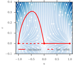
$$ \begin{cases} du = (u-u^3-\beta u v^2) dt + \sqrt{\epsilon}dW_u\\ dv = -(1+u^2)v dt + \sqrt{\epsilon}dW_v\,, \end{cases}$$

where $\beta$ is a parameter. For all values of $\beta$, the deterministic system has the two stable fixed points, $\varphi_-=(-1,0)$ and $\varphi_+=(1,0)$, and a unique unstable critical point $\varphi_s=(0,0)$. However it satisfies detailed balance only for $\beta=1$. To the right, the transition paths between the two stable fixed points is depicted in comparison to the heteroclinic orbit. The source code for this problem is available below.

Eggers model: Meta-stable climate regimes

Egger [J. Atm. Sc. 38, 12 (1981)] introduces the following SDE system as a crude model to describe weather regimes in central Europe:

$$\small \begin{aligned} da =& kb(U-\beta/k^2)\,dt - \gamma a\,dt + \sqrt{\epsilon} dW_a\,,\\ db =& -ka(U-\beta/k^2)\,dt + UH/k\,dt \\&- \gamma b\,dt + \sqrt{\epsilon} dW_b\,,\\ dU =& -bHk/2\,dt-\gamma(U-U_0)\,dt + \sqrt{\epsilon} dW_U\,. \end{aligned}$$

When $\epsilon$ is small, these equation exhibit metastability between a "blocked state" and a "zonal state". To the right, the transition paths between these two states is depicted in comparison to the heteroclinic orbit. The source code for this problem is available below.

Allen-Cahn/Cahn-Hilliard model: Phase separation and growth

Consider the SDE system

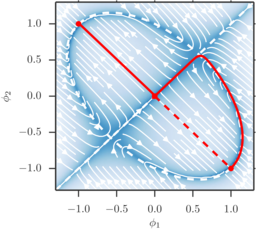
$$ d\phi= (\frac1\alpha Q (\phi-\phi^3) - \phi)dt + \sqrt{\epsilon} dW$$

with $\phi=(\phi_1, \phi_2)$ and the matrix $Q=((1,-1),(-1,1))$. This system does not satisfy detailed balance, as its drift is made of two gradient terms with incompatible mobility operators (namely $Q$ and $\textrm{Id}$). This model can be seen as a 2-dimensional reduction to a discretized version of the continuous Allen-Cahn/Cahn-Hilliard. When $\alpha$ is small, there exists a "slow manifold", comprised of all points where $Q(\phi-\phi^3)=0$ which is shown as a white dashed line to the right. On this manifold, the deterministic dynamics are of order $O(1)$, which is small in comparison to the dynamics of the $Q$-term, which are of order $O(1/\alpha)$. This suggests that for small enough $\alpha$ the transition trajectory will follow this slow manifold on which the drift is small, rather than the heteroclinic orbit, to escape the basin of the stable fixed points. This intuition is confirmed in the plot to the right. The source code for this problem is available below.

Genetic switch: A non-quadratic Hamiltonian

The algorithm can readily be applied to situations, where the Hamiltonian is non-quadratic. This is the case for example for birth-death-processes with a positive feedback loop, modeled as continuous time Markov process. The model

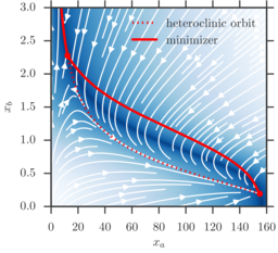
$$ \begin{aligned}H(\phi,\theta) &= \frac{a_1}{1+\phi_b^3}(e^{\theta_a}-1) + \phi_a(e^{-\theta_a}-1)\\&+ \frac{a_2}{1+\phi_a}(e^{\theta_b}-1) + \phi_b(e^{-\theta_b}-1)\end{aligned}$$

with $a_1=156, a_2=30$ was first defined by Roma et al. [Phys. Rev. E 71 (2005)] to model a genetic switching mechanism in molecular dynamics. The deterministic dynamics for this model follow along with minimizer and heteroclinic orbit for this setup are depicted to the right (zoomed into the "uphill" region).

Source code

Matlab source code with the generic algorithm and most of the examples above is available here

Relevant publications

T. Grafke, and E. Vanden-Eijnden, "Numerical computation of rare events via large deviation theory", Chaos 29 (2019), 063118 (link)
T. Grafke, T. Schäfer, and E. Vanden-Eijnden, "Long Term Effects of Small Random Perturbations on Dynamical Systems: Theoretical and Computational Tools", Fields Institute Communications, In: Recent Progress and Modern Challenges in Applied Mathematics, Modeling and Computational Science (Springer, New York, NY) (2017) (link)
T. Grafke, and E. Vanden-Eijnden, "Non-equilibrium transitions in multiscale systems with a bifurcating slow manifold" J. Stat. Mech 2017/9 (2017) 093208 (link)
T. Grafke, M. Cates, and E. Vanden-Eijnden, "Spatiotemporal Self-Organization of Fluctuating Bacterial Colonies", Phys. Rev. Lett. 119 (2017), 188003 (link)