Summary: Rare but extreme events are known to have dramatic influence on the statistics of turbulent flows, but are notoriously hard to handle both analytically and numerically. As alternative approach methods borrowed from field theory, most notably the instanton approach, allow for a direct computation of the most probable realizations of extreme events that dominate turbulent statistics. Not only can it be shown that the extreme events predicted by instanton analysis actually appear in turbulent flows, but we can furthermore predict the tail scaling of PDFs of turbulent quantities.
Instanton calculus and fluid dynamics
The term "instanton" was introduced in Yang-Mills theory as the classical solution of equations of motion in the Euclidean space with nontrivial topology in 1975. The main features of the instanton calculus as a non-perturbative method for the calculation of path integrals were highlighted on the example of 0+1 quantum mechanical systems in excellent reviews [1,2]. Although the physics of fluid dynamics have little overlap with Yang-Mills theory, importantly both are strongly coupled nonlinear systems. The comparison of quantum tunneling in a double well potential to Kramer's problem for escape rates in chemical reactions already exemplifies the connection between quantum mechanics and stochastic ordinary differential equations (SDEs). The calculus of instantons in fluid turbulence described by stochastic partial differential equations corresponds closely to the treatment of instantons in quantum field theory. However, naturally the question arises why a non-perturbative method like the instanton approach is especially promising for tackling the unsolved problem of turbulence.
Physically, the problem of turbulence is solved if one is able to derive from the equations full information about the probability density of velocity fluctuations or equivalently on correlation functions of any order. The natural approach known from kinetic theory is to find some closure approximation for terms involving higher correlations. In principle, this can be done by applying perturbation theory starting from the heat equation and introducing the nonlinearity as perturbation. This approach using renormalized perturbation theory (direct interaction approximation, DIA by Kraichnan) and/or renormalization group analysis was a major achievement of turbulence theory in the last century. However, from the current perspective it questionable, whether these approaches can describe the probability density functions (PDFs) of velocity fluctuations in the tail, which are extremely different from Gaussian fluctuations. The reason for this is the occurrence of nearly singular structures, such as vortex filaments for fluid turbulence and current sheets plasma turbulence, which are correlated over distances much larger than the dissipation scale and which cause strong departure from Gaussian behavior. Thus, for getting access to the tails of the velocity fluctuations PDF, non-perturbative approaches are required. The instanton approach is especially promising since the instantons are closely related to nearly singular events which form the skeleton of anomalous scaling and departure from Gaussianity, as already noted by Onsager.
The Martin-Siggia-Rose/Janssen/de Dominicis formalism
The functional integral description of stochastic systems started in the seventies with the Martin-Siggia-Rose/Janssen/de Dominicis (MSRJD) formalism [Martin, Siggia, Rose (1973), Janssen (1976)]. The method transforms the stochastic system into a functional integral representation. Although there is little hope to solve the path integral analytically, it is the starting point for systematic perturbation theory in stochastic dynamical systems (see especially [Taeuber (2014)] for applications in critical dynamics). It is also the basis for the instanton calculus for stochastic dynamical systems. To introduce the formalism, consider a stochastic partial differential equation (SPDE) of the form
in \(d\) space-dimensions, \(u\) having \(n\) components: \(u(x,t):\mathbb{R}^d \times [-T,0] \rightarrow \mathbb{R}^n\) and \(\eta\) being a Gaussian forcing with correlation
i.e. white in time and some correlation function \(\chi(r)\) in space.
In fluid dynamics applications, the exact form of the spatial correlation is often irrelevant and can be characterized solely by its amplitude \(\chi(0)\) and correlation length \(L\), where \(\chi(r)\) does not change significantly for \(x<L\) and decays to zero quickly for \(x>L\). Dimensionally, for example \(L=\sqrt{\chi(0)/\chi''(0)}\) (assuming the forcing is isotropic and \(\chi\) depends only on the scalar distance \(r\)). The forcing is then completely characterized by \(\chi(0)\) and \(\chi''(0)\). Furthermore, we will only be considering additive noise. The drift \(b\) in general is a nonlinear, non-gradient operator. A (quick) derivation (roughly following [Ivashkevich (1997)]) of the MSRJD formalism follows by considering the expectation of an observable \(O[u]\) and writing this expectation as a path integral taken over all noise realizations (using the fact that \(\eta\) is Gaussian and \(\delta\)-correlated in time). Keep in mind that the field \(u[\eta]\) has a functional dependence on the forcing \(\eta\) implicitly given by eqn. \((\ref{eq:spde})\):
where \(\langle{\cdot},{\cdot}\rangle\) is an appropriate inner product, e.g. \(L^2\). At this stage, we can consider the transformation of the noise paths to the paths of the field \(u\) given by \(\eta \rightarrow u\) given by (\ref{eq:spde}), hence \(\eta = \dot u - b[u]\). This coordinate transform leads to a Jacobian in \({\mathcal{D}}\eta = J[u] {\mathcal{D}} u\) with
Performing this coordinate change results in the Onsager-Machlup functional [Onsager, Machlup (1953), Machlup, Onsager (1953)]
This formulation is the starting point for directly minimizing the Lagrangian action
Since it is often more convenient to work with the original correlation function \(\chi\) instead of working with its inverse, we delay this coordinate change and introduce an auxiliary field \(\mu\) and obtain (by virtue of the Fourier transform, completion of the square) from (\ref{eq:pathint_mean}):
Now again considering the coordinate change \(\eta \rightarrow u\) we arrive at the path integral representation of \(O[u]\)
with the action function \(S[u,\mu]\) given by
also termed the Martin-Siggia-Rose/Janssen/de Dominicis (MSRJD) response functional. In many cases it can be shown explicitly that the Jacobian \(J(u)\) is not relevant to the discussion as it reduces to a constant, the value of which depending on the choice of either Itṓ or Stratonovich discretization (see e.g. [Ivashkevich (1997)]).
Two remarks should be added: (i) the change introducing an auxiliary field \(\mu\) to linearize the action with respect to the forcing is also known as Hubbard-Stratonovich transformation [Stratonovich (1957), Hubbard (1959)] and (ii) the MSRJD action \(S\) is closely related to classical limit of the Keldysh action [Keldysh (1964), Altland, Simons (2010), Kamenev (2011)].
The main idea of the instanton method is to compute the dominating contribution to this path integral via a saddle point approximation, i.e. by finding extremal configurations of the action functional (\ref{eq:action_MSR}).
Let us be more specific and consider an observable
for a scalar functional \(F[u]\), which is defined at the end point \(t=0\) of a path that started at \(-T<0\) (keeping in mind that we might be interested in the limit \(T\rightarrow \infty\)). The idea is that we observe an extreme event at \(t=0\) that has been created by the noise (and we give the noise infinite time to create the extreme event). In turbulent flow, for example, an extreme event of interest could be a large negative gradient of the velocity profile (i.e. \(F[u] = u_x \delta(x)\)), an event of high vorticity, an event of extreme local energy dissipation, etc.
Seeking a path integral representation of the probability distribution \({P}(a)\) for the events that fulfill \(F[u]=a\) at \(t=0\), we find
By now computing functional derivatives, we find
and it is easy to see that the saddle point equations (the instanton equations) are given by
where we have incorporated the Lagrange multiplier \(\lambda\) at the right hand side of the equation for \(\mu\) as a final condition equivalent to
A solution \((\tilde u, \tilde \mu)\) of this set of equations is termed the instanton configuration or instanton. It represents an extremal point of the action functional (\ref{eq:action_MSR}).
We want to make a few remarks on the instanton configuration and the structure of the chosen path integral representation:
- In the limit of applicability of the saddle point approximation, the instanton configuration corresponds to the most probable trajectory connecting the initial conditions to a final configuration which complies with the additional constraint defined by the observable \(O[u]\). In the language of quantum mechanics, it corresponds to the classical trajectory obtained for the limit \(\hbar \rightarrow 0\). For stochastic differential equations of the form (\ref{eq:spde}), we similarly need a smallness parameter to justify the saddle point approximation. This might either be the limit of vanishing forcing, \(\chi(0) \rightarrow 0\), or the limit of extreme events, \(|a| \rightarrow \infty\) (which corresponds to the limit \(|\lambda|\to \infty\), see discussion in sections \ref{ssec:FW} and \ref{ssec:instanton-equations}).
- It is instructive to apply a change of variables \((u,p) \equiv
(u,-i\mu)\). The response functional (\ref{eq:action_MSR}) can then be
written in terms of a Hamiltonian \(H[x,p]\),
\begin{eqnarray} \label{eq:action_MSR_xp} S[u,p] &=& \int\left(\langle{p},{\dot u}\rangle - H[u,p] \right)\,dt, \\ H[u,p] &=& \langle{p},{b[u]}\rangle + \frac12 \langle{p},{\chi p}\rangle. \end{eqnarray}The field variable \(u\) and the auxiliary field \(p\) then play the role of generalized coordinate and momentum for the Hamiltonian system defined by \(H[u,p]\). The instanton equations (\ref{eq:instanton_u_msr}), (\ref{eq:instanton_mu}) are the corresponding Hamiltonian equations of motion. We remark in particular that the Hamiltonian \(H[u,p]\) is a conserved quantity even if the original dynamical system (\ref{eq:spde}) is dissipative.
- In the above setup, note that the choice \(p=0\), \(\dot u=b[u]\) is a solution of the equations of motion with vanishing action, corresponding to a deterministic motion of the original dynamical system without any perturbation by noise. Since the action in general is always positive, \(S[u,p]\ge0\), this implies that a deterministic trajectory connecting the initial and final point (if it exists) will always be the global minimizer of the action functional.
- Another special solution with \(H=0\) is the choice \(p=-2\chi^{-1}b[u]\), which implies \(\dot u=-b\), i.e. the minimizer follows reversed deterministic trajectories. This choice is only consistent with the auxiliary equation of motion if \(\nabla_u b[u] = (\nabla_u b[u])^T\), as is easily verified by direct comparison between \(\dot p\) and equation (\ref{eq:instanton_mu}). This restriction is only fulfilled, if the drift term \(b[u]\) is gradient, \(b[u] = \nabla_u V[u]\), which forms an important sub-class of problems. Here, minimum action paths become minimum energy paths.
Application of the MSRJD formalism to extreme events in Burgers turbulence
The stochastically forced, viscous Burgers equation is given by
with a noise field \(\phi\) that is \(\delta\)-correlated in time and has finite correlation in space with correlation length \(L\). There are several motivations to study Burgers equation. A major motivation to study Burgers equation in the context of fluid turbulence is the fact that Burgers equation has a similar mathematical structure as the Navier-Stokes equations. As a one-dimensional equation, however, it is much easier to handle from both an analytical and computational point of view, in particular because it contains no non-local pressure term. There are important similarities (and equally important differences) between the phenomenology of turbulence in fluids described by the Navier-Stokes equations and Burgers turbulence (see e.g. [Bec, Khanin (2007)] for an overview of Burgers turbulence phenomenology). A major similarity between Burgers and the three-dimensional Navier-Stokes equations is the presence of a direct energy cascade: If energy is injected on large scales (or low Fourier modes), this energy is transported via the nonlinearity to small scales (corresponding to high Fourier modes) until the diffusive part of the equation becomes important and the energy is dissipated. Another major similarity between Burgers and Navier-Stokes turbulence is the existence of intermittency. This is manifest most strikingly in the existence of anomalous scaling for moments of velocity differences: The average increment of the velocity field on scale \(h\), \(\delta u(h) = \langle u(x+h/2)-u(x-h/2) \rangle\) and its moments \(\delta u_n(h) = \langle (u(x+h/2)-u(x-h/2))^n \rangle\) ("structure functions") exhibit a scaling of \(\delta u_n(h) \sim h^{\zeta_n}\). In contrast to the dimensional estimate \(\zeta_n = n/3\), the scaling exponents grow more slowly for \(n \rightarrow \infty\) for both Burgers and Navier-Stokes turbulence, a phenomenon that is believed to be connected to the intermittent nature of the flow.
In connection to this, a main quantity of interest in fluid systems are velocity gradients. High gradients are usually related to the most dissipative structures in the flow which govern the tails of the underlying probability distributions and structure functions. In the stochastically driven Burgers equation, we can immediately identify a difference in the behavior of positive and negative velocity gradients. For small viscosity \(\nu\) and moderate gradients, the solution will follow the characteristics of the equation, given by the nonlinearity \(uu_x\). This means that positive gradients will be smoothed out, whereas negative gradients will further steepen until they are so steep that the viscous term will start to counteract the advection and shocks are forming. This has important consequences for the tails of the velocity gradient probability distribution. Let us fix a point in space-time (for simplicity take \(x=0\) and \(t=0\)) and ask for the probability to observe a velocity gradient given by \(P(a) = P(u_x(0,0)=a)\). We are interested in extreme values for \(a\), either positive or negative. Consider first the case of \(a>0\). Then, the noise has to counteract the deterministic dynamics that drive the system back to smaller positive gradients. Intuitively, we will find that it is very difficult for the noise to generate such gradients, and we may expect the probability density to decay faster than a Gaussian. For sufficiently large \(a\), the scaling of the tail of the probability distribution should be characterized by the scaling of the associated minimizer of the Freidlin-Wentzell functional as we are clearly in a regime where we expect a large deviation principle to apply. The left tail of the velocity distribution is expected to have two different regimes: For small viscosity, it should be relatively easy for the system to generate moderate negative velocity gradients, simply following the deterministic dynamics of the nonlinearity that steepens the profile of the solution which would eventually lead to discontinuities in the velocity field if the system did not have any viscosity. Since the viscosity prohibits the occurrence of infinite gradients, once the gradient becomes too steep, it is again difficult for the noise to produce large negative gradients. Then, in the viscous tail of the distribution, again, the large deviation principle should be applicable and the scaling behavior is expected to be captured by the instanton (or minimizer of the Freidlin-Wentzell functional).
Following this intuition, there has been a considerable body of work devoted to the detail of the scaling of the function \(P(a)\). Concerning the right tail scaling, Gurarie and Migdal [Gurarie, Migdal (1996)] used the MSRJD formalism in order to derive the Euler-Lagrange equations associated with Burgers equation (\ref{eq:stochastic_burgers}) which are given by
These equations follow directly from (\ref{eq:instanton_u_msr}): simply set \(b[u] = -uu_x+\nu u_{xx}\) and compute \((\nabla_u b)^T = u\partial_x + \nu\partial_{xx}\) using integration by parts. In their work, focusing on the right tail of the probability distribution \(p\), Gurarie and Migdal introduced a finite-dimensional dynamical system approximating the solution of the Euler-Lagrange equation in order to predict that the distribution should decay much faster than Gaussian, i.e.
For the viscous left tail, Balkovsky et al. [Balkovsky, Falkovich, Kolokolov, et al. (1997)] applied the Cole-Hopf transform to the instanton equations and used a variety of careful approximations in order to predict that, in the limit \(a\rightarrow -\infty\), the scaling of \(p\) should behave like
These limiting results can be motivated by a rather simple phenomenological description: Velocity differences \(\delta u(h) = u(h/2)-u(-h/2)\) at the length scale \(h\) are increased by the (Gaussian) forcing according to the law \(\delta u^2 \sim \phi^2 t\). The breaking time of the shock structures can be estimated by \(t \sim L/\delta u\). Therefore, from \(P(\phi) \sim \exp(-\phi^2/\chi(0))\), one obtains \(P(\delta u) = \exp(-\delta u^3/(L \chi(0))\). Now, in smooth regions \(u_x \sim \delta u/h\), while for the shocks \(u_x \sim -\delta u^2/\nu\). We thus recover the exponents \(3\) and \(3/2\) for the right and left tail, respectively.
Yet, when comparing these limiting results to measurements in DNS, until recently, the role of the instanton for negative velocity gradients was unclear (and actually actively discussed among researchers). One numerical result obtained by Gotoh [Gotoh (1999)] via massive direct numerical simulations presented an estimate of the local scaling exponent of \(1.15\) for the probability distribution of the negative velocity gradients, which is surprisingly far away from the analytical prediction of \(3/2\). In 2001, Chernykh and Stepanov developed a numerical scheme to solve the instanton equations numerically [Chernykh, Stepanov (2001)]. This way they were able to show that all the approximations made by Balkovsky et al. leading to a scaling exponent of \(3/2\) were valid for the solution of these equations. These results rendered the discrepancy between DNS measurements and theoretical prediction even more in need of an explanation: In what sense are instanton configurations actually relevant in Burgers turbulence?
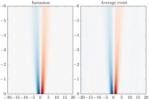
The answer to this question is given in the above figure: The instanton configurations themselves can be identified in realizations of turbulent Burgers flows by using an appropriate filtering technique \cite{grafke-grauer-schaefer:2013}. In other words, the instanton configuration is replicated exactly by averaging extreme velocity gradient events of stochastic turbulent Burgers simulations. Here, the \(x\)-axis denotes the spatial dimension, while the \(y\)-axis denots time: Approaching the final time, \(t\to0\), instanton and filtered event steepen into a shock localized in the origin. Note that there is virtually complete agreement between the instanton configuration and the stochastically averaged extreme event.
This agreement implies that the probability density function (PDF) of the velocity gradient is accessible by the instanton configuration if the associated gradient is extreme enough, in the sense that the saddle point approximation is justified. This works very nicely for low to medium Reynolds number events, as shown above, where the velocity gradient PDF is described completely in the low Reynolds number regime, and in the tails for higerh Reynolds numbers. The approximation fails if strong gradients become very probable, i.e. if the event is not extreme anymore.
Furthermore, in [Grafke, Grauer, Schaefer, Vanden-Eijnden (2015)] we were able to show that for the parameters chosen in Gotoh's simulation, the scaling exponent of the velocity gradient given by the (numerical) solution of the instanton equations is actually \(1.16\), hence very close to the measured value. The regime in which these numerical simulations were carried out was simply not yet in the range of validity of the asymptotic analysis that was carried out analytically, but nevertheless already in a regime where the instanton approximation is valid. The resolution of this 'puzzle' is encouraging and gives hope that instantons are relevant in a wide-range of fluid dynamics and can help to answer many open questions in the field.
Relevant publications
-
T. Grafke, R. Grauer, and T. Schäfer, "The Instanton Method and its Numerical Implementation in Fluid Mechanics", J. Phys. A: Math. Theor. 48 (2015), 333001
-
T. Grafke, R. Grauer, T. Schaefer and E. Vanden-Eijnden, "Relevance of instantons in Burgers turbulence", EPL 109 (2015), 34003
-
T. Grafke, R. Grauer and T. Schaefer, "Instanton filtering for the stochastic Burgers equation", J. Phys. A 46 (2013), 62002
-
T. Grafke, R. Grauer, and S. Schindel, "Efficient Computation of Instantons for Multi-Dimensional Turbulent Flows with Large Scale Forcing", Commun. Comp. Phys. 18 (2015), 577