Models for Turbulent Pipe Flow

I have proposed modeling transitional pipe flow as an excitable and bistable medium⁰ ¹ ². The models are presented in two variables, turbulence intensity and mean shear, that evolve according to established properties of transitional turbulence described below. A continuous model captures the essence of the puff-slug transition as a change from excitability to bistability. A discrete model and a stochastic PDE model additionally incorporate turbulence that is locally transient. These models reproduce almost all large-scale features of transitional pipe flow. In particular they captures metastable localized puffs, puff splitting, slugs, localized edge states, a continuous transition to sustained turbulence via spatiotemporal intermittency (directed percolation), and a subsequent increase in turbulence fraction towards uniform, featureless turbulence.
You may wish to visit the comparison gallery.

Two Variables

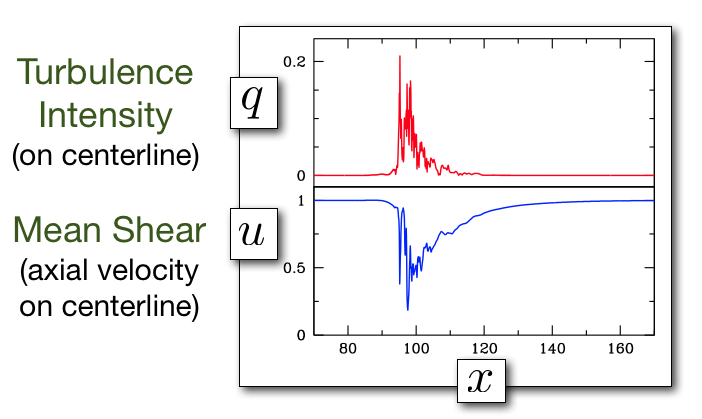
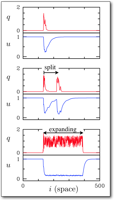
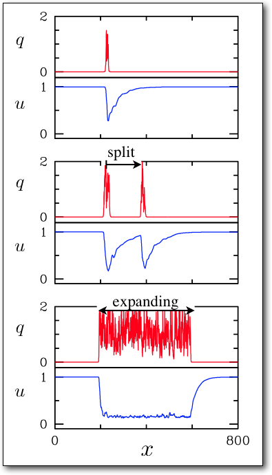
Shown below are the instantaneous turbulent fluctuations and the mean shear profiles from direct numerical simulation (DNS) of a turbulent puff at Re=2000. (The turbulent fluctuations are here simply the magnitude of transverse velocity. The mean is shear profiles are instantaneous azimuthal averages of streamwise velocity.)

Two scalar variables, q and u, depending only on streamwise coordinate x are obtained by sampling the above fields on the centerline. The axial velocity on the centerline provides a convenient proxy for the mean shear.

Physical Features

Models are based on the following established properties of transitional turbulence. Most of these features are seen in the figure below. The first four properties are contained in Wygnanski et al.³ ⁴,Sreenivasan et al.⁵, and other “classic” works. The last two properties, and especially the crucial final property, have been understood only more recently⁶ ⁷.

Sharp upstream front, where turbulent energy is extracted from fully developed, or nearly fully developed, laminar shear. This results in a rapid change in the mean shear. This is seen in on the left side of turbulent patches in all cases (a) – (c).
Reverse transition on downstream side of puff. Turbulence cannot be sustained in modified shear profile. This occurs at the right side of turbulent patches in (a) and (b).
No reverse transition on downstream side of slug. Turbulence can be sustained with modified shear profile. Slugs expand to arbitrary streamwise length, as seen in (c).
Slow recovery following excitation. The shear recovers slowly following the decay of turbulence. This is seen in on slow recovery of the centerline velocity in of the left side in all cases.
State of recovery controls susceptibility to re-excitation. It is not possible to re-excite a turbulent puff until the shear profile has recovered sufficiently. This results in a minimum spacing between puffs seen in (b).
Turbulence is locally transient. In localized regions of space turbulence is a chaotic saddle, not a chaotic attractor. It is not possible to see this effect in the figures.

Figure shows variables q and u from direct numerical simulation of transitional pipe flow. (a) puff at Re=2000, (b) pair of puffs immediately following a splitting event at Re=2275, (c) expanding slug flow at Re=3200. These same states are observed experimentally⁸ ⁹.

Puff-Slug Transition

The following PDE model capture all of the above physical properties, except the last.

The parameter r plays the role of Reynolds number. The most essential point is that these equations capture the difference between puffs and slugs as a difference between excitability and bistability. The transition occurs at r = r_c, where r_c is easily computable. Further details of these equations can be found in papers and talks here. It is probably useful to understand basic properties of excitable media¹⁰ ¹¹.

Puff Regime – excitability

There is a reverse transition on the downstream side of model puffs. This gives puffs a finite, selected streamwise width. They propagate at a selected speed determined by the upstream front.

Slug Regime – bistability

There is no reverse transition on the downstream side of model slugs. The system is locally bistable. The upstream and downstream fronts have different selected speeds and the slugs can expand to arbitrary streamwise length.

In each of the above figures, the left plot shows snapshots of variables q and u as function of x, as in the simulation of pipe flow. The right plot shows these snapshots as curves in the u-q phase plane with arrows indicating increasing x. Blue and red curves indicate the u- and q-nullclines, respectively.

Locally Transient Chaos The above PDE model captures the essence of the puff-slug transition, but misses the crucial property of locally transient chaos (chaotic saddle). Here two approaches have been used to incorporate this while keeping with a two-variable description.
Map Model (Discrete) Space and time are discrete. The u-equation is obtained an Euler time step of the PDE model. The q-equation uses a tent map (given by the function F) to generate locally transient chaotic dynamics. The dynamics is deterministic. Noise Model (SPDE) Multiplicative noise is added to the q-equation. The dynamics is random. These models capture nearly all large-scale features of transitional pipe flow. Below are illustrations of puffs, puff-splitting, and slugs in the two models. Further comparisons can be seen here.
Map Model	Noise Model
The left figure shows states from simulations of the map model: metastable puff at R=2000, puff splitting at R=2100, and slug at R=3200. The right figure shows states from simulations of the SPDE model: metastable puff at r=0.7, puff splitting at r=0.94, and slug at r=1.2. Full details, including values of other model parameters, can be found in detailed publications.